ASPHALTIC EQUATIONS
& EXAMPLE CALCULATIONS
SCOPE
This IM describes the equations associated with asphaltic materials. In addition, there are a number of example calculations showing how to determine various properties.
NAMING CONVENTION
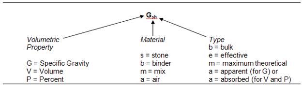
DEFINITIONS
|
Pa |
= |
% of air voids in compacted hot mix asphalt mixture (percent of total volume) Lab Voids for gyratory specimens or Field Voids for cores |
|
|
|
|
|
Pb |
= |
% of asphalt binder in the hot mix asphalt mixture |
|
|
|
|
|
Pb(RAP) |
= |
% of asphalt binder in RAP material |
|
|
|
|
|
Pb(add) |
= |
% of virgin asphalt binder needed to add to the mix to achieve the total intended binder content |
|
|
|
|
|
Pb(added) |
= |
% of virgin asphalt binder in the hot mix asphalt mixture. Does not include the asphalt binder from the RAP |
|
|
|
|
|
Ps |
= |
% of combined aggregate in the hot mix asphalt mixture |
|
|
= |
100 – Pb - other non-aggregate components |
|
|
|
|
|
Pba |
= |
% of asphalt binder absorbed by aggregate, aggregate basis |
|
|
|
|
|
Pba (mix) |
= |
% of asphalt binder absorbed by aggregate, mix basis |
|
|
|
|
|
Pbe |
= |
effective asphalt binder, %, mixture basis |
|
|
|
|
|
% Abs |
= |
% water absorption of the individual or combined aggregate |
|
|
|
|
|
ABS |
= |
fraction of water absorption of the individual or combined aggregate |
|
|
= |
% Abs/100 |
|
|
|
ABS is always used in the calculations rather than % Abs. |
|
|
|
|
|
Gsa |
= |
apparent specific gravity of the aggregate |
|
|
|
|
|
Gse |
= |
effective specific gravity of the combined aggregate |
|
|
|
|
|
Gsb |
= |
bulk specific gravity of the aggregate (dry basis) |
|
|
|
|
|
Gsb(SSD) |
= |
bulk specific gravity of the aggregate (SSD basis) |
|
|
|
Used for Portland Cement Concrete NOT ASPHALT!!! |
|
|
|
|
|
Gb |
= |
specific gravity of the asphalt binder at 25°C (77°F) |
|
|
|
|
|
Gb (effective) |
= |
effective specific gravity of the combined new and recycled asphalt binder at 25°C (77°F) |
|
|
|
|
|
% New AC |
= |
percentage of the total binder that is virgin (not from RAM) |
|
|
|
|
|
Gmm |
= |
maximum specific gravity of the hot mix asphalt mixture. Often referred to as the Rice specific gravity, solid specific gravity or solid density. |
|
|
|
|
|
Gmb |
= |
bulk specific gravity of compacted hot mix asphalt mixture |
|
|
|
|
|
Gmb(measured) |
= |
Gmb of gyratory specimen as determined from test procedure in IM 321 |
|
|
|
|
|
Gmb(corrected) |
= |
corrected Gmb of gyratory specimen at Ndes, also called Lab Density. |
|
|
|
Gmb(corrected) and Gmb(measured) will be the same when compacting to Ndes so no correction is necessary. |
|
|
|
|
|
Gmb(field core) |
= |
bulk specific gravity of pavement cores (also Gmb(field) or Field Density) |
|
|
|
|
|
VMA |
= |
% voids in mineral aggregate, (percent of bulk volume), compacted mix |
|
|
|
|
|
Vt |
= |
design target air voids, % |
|
|
|
|
|
VFA |
= |
% voids filled with asphalt binder |
|
|
|
|
|
Nini |
= |
Number of gyrations used to measure initial compaction. |
|
|
|
|
|
Ndes |
= |
Number of gyrations used to measure design compaction. Gmb for Lab |
|
|
|
Density is determined at Ndes. |
|
|
|
|
|
Nmax |
= |
Number of gyrations used to measure maximum compaction. |
|
|
|
|
|
Nx |
= |
Level of compaction, where x is the number of gyrations. |
|
|
|
|
|
R |
= |
temperature correction multiplier obtained from IM 350 Table 2 App. A |
|
|
|
|
|
dt |
= |
density of water at test temperature, g/cc |
|
|
|
|
|
hmax |
= |
the height of the specimen at Nmax, mm |
|
|
|
|
|
hdes |
= |
the height of the specimen at Ndes, mm |
|
|
|
|
|
hx |
= |
the height of the specimen at any gyration level Nx, mm |
|
|
|
|
|
Cx |
= |
percent of compaction expressed as a percentage of Gmm |
|
|
|
Where x is the number of gyrations (this is normally Nini or Nmax) |
|
|
|
|
|
S |
= |
slope of the compaction curve |
|
|
|
|
|
FT |
= |
Film Thickness, microns |
|
|
|
|
|
SA |
= |
Surface Area, m2/kg |
|
|
|
|
|
F/B |
= |
Filler/Bitumen Ratio also called Fines/Bitumen Ratio |
|
|
|
|
|
sn-1 |
= |
Sample Standard Deviation |
|
x̄ |
= |
sample average |
FORMULAS
All calculations shown have been rounded for ease of presentation. Normally calculations will involve maintaining more significant figures throughout the intermediate calculations and only rounding the final result. The values generated by the software specified by the DOT will be the accepted results for reporting purposes.
All specific gravity calculations will be reported to 3 decimal places. Binder content is reported to 2 decimal places. Percent voids, VMA and VFA are reported to 1 decimal place.
Unless noted as otherwise, the following information is given to perform the calculations for a mix not containing RAS. Any additional needed information will be provided with the sample calculation.
|
Pb = 5.75% |
Gsa = 2.667 |
Gmb (field) = 2.215 |
|
|
|
|
|
Ps = 100 – 5.75 = 94.25% |
Gse = 2.659 |
Gmb |
|
|
|
|
|
% Abs = 1.39 |
Gsb = 2.572 |
Gmb (corrected) = 2.273 |
|
|
|
|
|
ABS = 1.39/100 = 0.0139 |
Gsb(SSD) = 2.608 |
% RAP = 10.0% |
|
|
|
|
|
Gb = 1.031 |
Gmm = 2.438 |
Pb(RAP) = 5.00% |
|
|
|
|
|
% minus #200 (75 μm) sieve = 5.0% |
|
|
VOLUMETRIC EQUATIONS
To convert the specific gravity of asphalt binder from one temperature to another, the following two equations are used.
|
|
|
|
|
|||||||||||
|
|
|
|
|
|
||||||||||
|
|
|
|
|
|||||||||||
|
|
|
|
|
|
||||||||||
|
Gb (effective) with RAM |
|
|
||||||||||||
|
|
|
|
|
|
||||||||||
|
% Abs |
|
|
|
|
||||||||||
|
|
|
|
|
|
||||||||||
|
|
|
|
|
|
||||||||||
|
|
|
|
||||||||||||
|
|
|
|
|
|
||||||||||
|
|
|
|
|
|
||||||||||
|
|
Where: |
Wa = Saturated-Surface-Dry (SSD) weight of coarse portion, 1315.7 g |
||||||||||||
|
|
|
Wb = Saturated-Surface-Dry (SSD) weight of fine portion, 690.3 g |
||||||||||||
|
|
|
Wc = Combined dry weight of coarse and fine portion, 2000.0 g |
||||||||||||
|
|
|
|
|
|
||||||||||
|
% Abs(combined) |
|
|
||||||||||||
|
|
|
|
|
|
||||||||||
|
|
|
|
||||||||||||
|
|
|
|
|
|
||||||||||
|
|
Where: |
% Abs1 = 0.67% |
Ps1 = 50% |
|||||||||||
|
|
|
% Abs2 = 1.23% |
Ps2 = 5% |
|||||||||||
|
|
|
% Abs3 = 2.21% |
Ps3 = 45% |
|||||||||||
|
|
|
|
|
|
||||||||||
|
Gsa |
|
|
|
|||||||||||
|
|
|
|
|
|
||||||||||
|
|
|
|
|
|
||||||||||
|
|
Where: |
W = Weight of dry sample, 2000.0 g |
||||||||||||
|
|
|
W1 = Sample weight of pycnometer filled with water at test temperature, 6048.0 g |
||||||||||||
|
|
|
W2 = Sample weight of pycnometer filled with water and sample, 7298.1 g |
||||||||||||
|
|
|
R = Multiplier to correct temperature to 77°F = 1.0000 @ 77°F |
||||||||||||
|
|
|
|
|
|
||||||||||
|
|
|
|
|
|
||||||||||
|
Gsb |
|
|
||||||||||||
|
|
|
|
||||||||||||
|
|
|
|
||||||||||||
|
Gsb (combined) |
|
|
||||||||||||
|
|
|
|
|
|
||||||||||
|
|
|
|
|
|
||||||||||
|
|
|
|
|
|
||||||||||
|
|
Where: |
Ps1 = 50.0% |
Gsb1 = 2.657 |
|
||||||||||
|
|
|
Ps2 = 5.0% |
Gsb2 = 2.642 |
|
||||||||||
|
|
|
Ps3 = 45.0% |
Gsb3 = 2.640 |
|
||||||||||
|
|
|
|
|
|
||||||||||
|
Gse |
|
|
|
|||||||||||
|
|
|
|
|
|
||||||||||
|
|
|
|
|
|
||||||||||
|
Gmm |
|
|
|
|||||||||||
|
|
|
|
|
|
||||||||||
|
|
|
|
|
|
||||||||||
|
|
Where: |
W = Sample weight of sample, 2020.0 g |
||||||||||||
|
|
|
W1 = Sample weight of pycnometer filled w/water at test temperature, 6048.0 g |
||||||||||||
|
|
|
W2 = Sample weight of pycnometer filled w/water and sample, 7239.5 g |
||||||||||||
|
|
|
R = Multiplier to correct temperature to 77°F = 1.0000 @ 77°F |
||||||||||||
|
|
||||||||||||||
|
To correct the density of water to 77°F the R multiplier is used. The value of R is given in the tables in IM’s 350 and 380 for temperatures from 60 to 130°F. R is calculated as follows: |
||||||||||||||
|
|
|
|
|
|
||||||||||
|
R |
|
|
|
|||||||||||
|
|
|
|
|
|
||||||||||
|
|
|
|
|
|
||||||||||
|
|
Where: |
dt = density of water at temperature t = 0.99707 g/cc at 77°F. |
||||||||||||
|
|
|
|
|
|
||||||||||
|
Gmb (or Gmb (measured)) |
|
|
||||||||||||
|
|
|
|
|
|
||||||||||
|
|
|
|
|
|
||||||||||
|
|
Where: |
W1 = Sample Dry weight, 4800.0 g |
||||||||||||
|
|
|
W2 = Sample weight in water, 2727.7 g |
||||||||||||
|
|
|
W3 = Sample weight in air, SSD, 4805.6 g |
||||||||||||
|
|
|
|
|
|
||||||||||
|
|
|
|
|
|
||||||||||
|
Pa (lab voids) |
|
|
||||||||||||
|
|
|
|
|
|
||||||||||
|
|
|
|
|
|
||||||||||
|
%Gmm (field core) |
|
|
||||||||||||
|
|
|
|
|
|
||||||||||
|
|
|
|
|
|
||||||||||
|
Pa (field voids) |
|
|
||||||||||||
|
|
|
|
|
|
||||||||||
|
|
|
|
|
|
||||||||||
|
VMA |
|
|
||||||||||||
|
|
|
|
|
|
||||||||||
|
|
|
|
|
|
||||||||||
|
VFA |
|
|
||||||||||||
|
|
|
|
|
|
||||||||||
|
|
|
|
|
|
||||||||||
|
Pba |
|
|
||||||||||||
|
|
|
|
|
|
||||||||||
|
|
|
|
|
|
||||||||||
|
Pbe |
|
|
||||||||||||
|
|
|
|
|
|
||||||||||
|
Pba (mix) |
= Pb - Pbe |
|||||||||||||
|
|
|
|
|
|
||||||||||
|
F/B (fines/bitumen) |
|
|
||||||||||||
|
|
|
|
|
|
||||||||||
|
|
|
|
|
|
||||||||||
|
|
Where: |
Total % of minus #200 (75 μm) includes both virgin aggregate and RAM when used |
||||||||||||


GYRATORY EQUATIONS
If compacting to Nmax a correction to the measured Gmb must be performed. The corrected Gmb (Gmb (corrected)) is then used in the calculations for Pa (lab voids) and VMA.
To correct Gmb from the measured value at Nmax to the corrected value at Ndes:
|
Gmb (corrected) |
(lab density) |
|
|
|||||
|
|
|
|
|
|||||
|
|
|
|
|
|||||
|
|
Where: |
hmax = 117.5 mm (the height at Nmax) and hdes = 119.4 (the height at Ndes) |
||||||
|
|
|
|
|
|||||
|
To find the percent of maximum specific gravity (%Gmm) at a specific gyration (Nx): |
||||||||
|
|
|
|
|
|||||
|
|
|
|
|
|||||
|
Cx |
(%Gmm) |
|
||||||
|
|
|
|
|
|||||
|
|
|
|
|
|||||
|
|
|
Nini = 8 gyrations |
h8 = 135.4 mm |
|||||
|
|
Given: |
Ndes = 109 gyrations |
h109 = 119.4 mm |
|||||
|
|
|
Nmax = 174 gyrations |
h174 = 117.5 mm |
|||||
|
|
|
|
|
|||||
|
|
|
|
|
|||||
|
C8 |
|
|
||||||
|
|
|
|
|
|||||
|
|
|
|
|
|||||
|
C109 |
|
|
||||||
|
|
|
|
|
|||||
|
|
|
|
|
|||||
|
C174 |
|
|
||||||
|
|
|
|
|
|||||
|
|
|
|
|
|||||
|
To find the slope of the gyratory compaction curve: |
||||||||
|
|
|
|
|
|||||
|
|
|
|
|
|||||
|
S |
|
|
|
|||||
|
|
|
|
|
|||||
|
|
|
|
|
|||||
|
|
Where: |
Cmax and Cini are expressed as decimals. |
||||||
RAP FORMULAS
To determine the percent of asphalt binder to add to a mix containing RAP (Pb(add)) to achieve the total intended Pb shown on the JMF (this the value to which the plant controls are set):
|
Pb(add) |
|
|
|
|
|
|
|
|
|
|
|
|
|
|
|
|
|
|
To determine the percent of aggregate contributed by the RAP in the total aggregate blend:
|
|
|
|||
|
|
|
|||
|
|
|
|||
|
|
|
|||
|
|
|
|||
|
|
|
|||
|
To determine the actual percent virgin aggregate in the total aggregate blend containing RAP: |
||||
|
|
|
|||
|
|
|
|||
|
|
|
|||
|
|
|
|||
|
|
|
|||
|
|
|
|||
|
|
|
|||
|
To determine the total percent asphalt binder in a mix containing RAP: |
||||
|
|
|
|||
|
Total Pb |
= |
|||
|
|
|
|||
|
|
|
|||
|
|
|
|||
|
|
|
|||
|
|
|
|||
|
|
Where: |
Pb(added) is the actual percent of virgin asphalt binder added to the mix from the tank stick, flow meter or batch weights - not the Pb(add) determined above which is the original determination on the JMF. |
||
|
|
|
|||
FRICTION AGGREGATE CALCULATIONS
Percent Retained on #4 Sieve:
% +#4 Frictional aggregate![]()
Example: The aggregate blend contains 20% quartzite as the Type 2 friction class aggregate, the quartzite gradation shows 90% retained on the #4 sieve, and the combined gradation of the blend shows 60% retained on the #4 sieve:
% +#4 frictional aggr. in total blend = +#4
Type 2 ![]()
Percent Passing the #4 Sieve:
% −#4 Type 2 aggregate ![]()
Example: For a single Type 2 aggregate:
Quartzite Type 2 aggregate is 20% of the total blend and has 58% passing the #4 sieve. The combined gradation of the total blend has 65% passing the #4 sieve.
% −#4 Type 2 in the total
blend
![]()
If more than one Type 2 aggregate is included in the blend the gradations of the Type 2 aggregates must be combined first in the numerator to determine the percent passing the #4 sieve for the Type 2 aggregate as shown in the following example.
Example: For multiple Type 2 aggregates:
Three quartzite aggregates are included in the total blend. The graded quartzite aggregate is 20% of the total blend and has 58% passing the #4 sieve. The quartzite man sand is 10% of the total blend and has 100% passing the #4 sieve. The quartzite chip is 5% of the total blend and has 5% passing the #4 sieve. The combined gradation of the total blend has 65% passing the #4 sieve.
The % Type 2 in the total blend combined −#4 is:
% −#4 Type 2 in the total blend ![]()
Fineness Modulus
The fineness modulus of the Type 2 (FMType2) material is expressed as 600 minus the total of the percents passing each of the six sieves from the #4 to the #100 sieves divided by 100 and then multiplied by the percentage of Type 2 aggregate in the total blend expressed as a decimal.
![]()
Where:
Px is the percent passing sieve #x (x = #4, #8, #16, #30, #50, and #100)
PType 2 is the percent of Type 2 aggregate in the total blend expressed as a decimal
When more than one Type 2 aggregate is included in the total blend the gradations of the Type 2 aggregates must be combined first to determine the percent passing each of the six sieves for the total Type 2 aggregate as shown in the following example.
Example:
Given: The following gradations of the three Type 2 aggregates and the percentages in the total blend:
|
Percent Passing |
3/4 |
1/2 |
3/8 |
#4 |
#8 |
#16 |
#30 |
#50 |
#100 |
#200 |
|
20% Graded Quartzite |
100 |
98 |
78 |
58 |
48 |
38 |
28 |
18 |
8.0 |
4.0 |
|
10% Quartzite Man Sand |
|
|
|
100 |
75 |
52 |
33 |
22 |
7.0 |
2.0 |
|
5% Quartzite Chip |
100 |
95 |
35 |
5.0 |
4.5 |
4.0 |
3.5 |
3.0 |
2.0 |
1.0 |
The total percent Type 2 quartzite in the total blend is 20+10+5=35%
To combine the gradations of the Type 2 aggregates, multiply the percent passing each sieve (#4 to #100) for each aggregate by the percent of that aggregate in the total blend, sum the results individually for each sieve then divide the sum by the total percent Type 2 in the total blend as shown below. Express the result to two significant figures.
Combined gradation of the Type 2 for the #4 sieve: ![]()
Perform this same calculation for each of the other five sieves, #8, #16, #30, #50 and #100
|
Percent Passing |
3/4 |
½ |
3/8 |
#4 |
#8 |
#16 |
#30 |
#50 |
#100 |
#200 |
|
Total Type 2 Combined |
|
|
|
62 |
50 |
37 |
26 |
17 |
6.9 |
|
![]()
FILM THICKNESS EXAMPLE:
The surface area (SA) is found by taking the % Passing times the Surface Area Coefficient. The Surface Area for the material above the #4 sieve is a constant 0.41. The total surface area is found by adding all of the individual surface area values.
|
SA |
(for each sieve) |
|
|||
|
|
|
|
|
||
|
|
|
|
|||
|
|
|
|
|
||
|
|
Where: |
The Surface Area Coefficients are constants. |
|||
|
|
|
|
|
||
|
FT |
(Film Thickness) |
|
|
||
MISCELLANEOUS
|
Optimum Pb |
|
||||||||||
|
|
|
||||||||||
|
|
|
||||||||||
|
|
Where: |
Target voids = 4.0 |
|||||||||
|
|
|
|
|||||||||
|
|
|
Pb |
Pa |
|
|||||||
|
|
(low Pb =) |
4.75 |
5.5 |
(= high voids) |
|||||||
|
|
(high Pb =) |
5.75 |
3.0 |
(= low voids) |
|||||||
|
|
|
6.75 |
1.2 |
|
|||||||
|
|
|||||||||||
|
Since the target voids of 4.0% falls between 5.5 and 3.0 they are the high voids and low voids respectively. The asphalt contents associated with those voids are used as the low Pb and high Pb respectively. |
|||||||||||
|
|
|||||||||||
|
|
|
||||||||||
|
|
|
||||||||||
|
|
|
||||||||||
|
% Moisture |
|
||||||||||
|
|
|||||||||||
|
|
|||||||||||
|
|
Where: |
Wet Wt. Sample = 2100.0 g |
|||||||||
|
|
|
Dry Wt. Sample = 2000.0 g |
|||||||||
|
|
|||||||||||
|
|
|||||||||||
|
|
|
||||||||||
|
|
|||||||||||
|
|
|||||||||||
|
To adjust the height of a Gmb specimen to reach the intended height, the following equation is used. |
|||||||||||
|
|
|||||||||||
|
Adjusted sample weight |
|
||||||||||
|
|
|||||||||||
|
|
|||||||||||
|
|
|
||||||||||
|
|
|||||||||||
|
|
|||||||||||
|
Gsb (from Gsb(SSD)) |
|
|
|||||||||
|
|
|||||||||||
|
|
|||||||||||
|
|
|
|
|||||||||
|
|
|||||||||||
|
|
|||||||||||
|
Min. Pb |
|
||||||||||
|
|
|||||||||||
|
|
|||||||||||
|
|
|
||||||||||
|
|
|||||||||||
|
|
|||||||||||
|
You have 13,000 grams of aggregate and 650 grams of asphalt binder. Determine the asphalt binder content (Pb) of the mixture. |
|||||||||||
|
|
|||||||||||
|
Pb |
|
|
|||||||||
|
|
|||||||||||
|
|
|||||||||||
|
|
Where: |
Wb = Weight of the asphalt binder, g |
|||||||||
|
|
Ws = Weight of the aggregate, g |
||||||||||
|
|
Pb = Percent binder of the mix, mix basis |
||||||||||
|
|
|||||||||||
|
You have 13,000 grams of aggregate. You want to prepare a mixture having 5.5% asphalt binder content based on the total mix. Determine the weight of the asphalt binder you need to add to the aggregate. |
|||||||||||
|
|
|||||||||||
|
Wb |
|
|
|||||||||
|
|
|||||||||||
|
|
|||||||||||
|
|
Where: |
Wb = Weight of the added binder, mix basis, g Ws = Weight of the aggregate, g |
|||||||||
|
|
|||||||||||
QUALITY INDEX (QI) EXAMPLE %Gmb Method:
(This example is applicable for calculating outliers for Gmb and gradation)
For use on projects not using the PWL specifications
|
|
Given: |
lab. lot average Gmb(corrected) = 2.408 |
|||||||||
|
|
field Gmb of individual cores: 2.319, 2.316, 2.310, 2.298, 2.242, 2.340, and 2.345. |
||||||||||
|
|
% of lab density = 94%, 95%, or 96%. For this example 95% is used. |
||||||||||
|
|
|
|
|||||||||
|
Determine the average field density (Gmb) of the seven cores. |
|||||||||||
|
|
|
|
|||||||||
|
x̄ |
|
||||||||||
|
|
|
|
|||||||||
|
|
|
|
|||||||||
|
The sample standard deviation is determined as follows: |
|||||||||||
|
|
|
|
|||||||||
|
sn-1 |
|
|
|||||||||
|
|
|
|
|||||||||
|
|
|
|
|||||||||
|
|
Where: |
x = individual sample value |
|
||||||||
|
|
n = number of samples |
|
|||||||||
|
|
x̄ = average of all samples |
|
|||||||||
|
|
|
|
|||||||||
|
The Quality Index for density shall be determined according to the following calculation: |
|||||||||||
|
|
|||||||||||
|
|
|
||||||||||
|
|
|||||||||||
|
|
|||||||||||
|
QI |
|
||||||||||
|
|
|||||||||||
|
|
|||||||||||
|
The QI is less than 0.72. Check for outliers. To test for a suspected outlier result, apply the appropriate formula. |
|||||||||||
|
|
|||||||||||
|
|
|
|
|||||||||
|
|
|||||||||||
|
|
|||||||||||
|
|
|
|
|||||||||
|
|
|||||||||||
|
|
|||||||||||
|
The highest density or lowest density shall not be included if the suspected outlier result is more than 1.80 for seven samples. The quality index shall then be recalculated for the remaining six samples. |
|||||||||||
|
|
|||||||||||
|
The suspected low outlier result is greater than 1.80 for seven samples, therefore the core with the lowest density, 2.242, is an outlier. |
|||||||||||
|
|
|||||||||||
|
Recalculate the QI for the remaining six densities (excluding the outlier). |
|||||||||||
|
|
|||||||||||
|
Avg. Gmb (field lot)(new) |
= 2.321 |
= σn-1 (new) |
= 0.018 |
||||||||
|
|
|||||||||||
|
QI(new) |
|
||||||||||

GRADATION EXAMPLE (Combined Gradation):
Assume the proportions of the individual aggregates are as follows: 50% ¾”
Minus, 5% ⅜” Chips, and 45% Nat. Sand. Then using the following
gradations for the individual aggregates, determine the combined gradation.
To determine the combined gradation, take each individual material % Passing times the percentage of that material in the blend. For example, take the 50% of the 3/4” Minus material times the % Passing for that material.
3/4” Minus Portion % Passing #200 sieve: ![]()
Do the same thing with each of the other aggregates and sieve sizes to obtain the following:

Next, sum the individual sieve sizes to get the combined gradation. This will result in the following combined gradation.
![]()
BATCHING EXAMPLE:
You have been directed to prepare a 13,000-gram batch of aggregate composed of the aggregates used above with the same proportions. The ¾” Minus has been split into four size fractions by sieving on the 12.5 mm, 9.5 mm and 4.75 mm sieves. The ⅜” Chip has been split into three size fractions by sieving on the 9.5 mm and 4.75 mm sieves. The Nat. Sand is one size fractions passing the 4.75 mm sieve. Complete the following batching sheet by determining the mass of each aggregate needed, the percentage of each size fraction and the weight of each size fraction.
Weight ¾” Minus @ 50% = __________ grams

Weight ⅜” Chip @ 5% = __________grams
Weight Nat. Sand @ 45% = __________grams

The weight of each material is found by taking the percentage of the blend each material is times the total batch weight. For example, the weight of the ¾” Minus is found by taking 50% of the 13,000 gram batch, or 6,500 grams.
The % In Size Fraction column is found by subtracting the % Passing from one size by the previous size % Passing. For example, the % In Size Fraction for the –19 + 12.5 Size Fraction is found by subtracting 90% Passing the 12.5 mm sieve from 100% Passing the 19 mm sieve. This process is repeated for each size fraction. The last line in the % In Size Fraction column is found by adding each of the individual values above it. The total should be 100.0%.
The Weight Needed Each Fraction is found by taking the % In Size Fraction value and multiplying it by the total mass of that aggregate. For example, for the ¾” Minus material, there is 10% in the –19 + 12.5 size fraction. Take this 10% times the mass of 6,500 grams to get the Weight Needed value of 650 grams.
The Cumulative Weight is found by taking the first value in the Weight Needed column and placing it in the first spot for the Cumulative Weight column. For example, there was 650 grams needed in the previous example. This value would go on the first line of the Cumulative Weight column. Each successive line requires adding the corresponding Weight Needed value with the previous Cumulative Weight value. Below are the solutions for the example shown above.
Weight ¾” Minus @ 50% = 6500.0 grams
Weight ⅜” Chip @ 5% = 650.0 grams
Weight Nat. Sand @ 45% = 5850.0 grams
The Cumulative Weight at the end of the batching should always equal the desired total batch weight.
Determination of Tons of Asphalt Binder Used
Determine the tons of asphalt binder used in the mix for a given day using the following information:
Weights of all Binder @ 60°F = 8.67 lbs./gal.
Beginning tank stick 18,000 gal. @ 296°F
28.0 tons Binder hauled in during the day’s run
Ending tank stick 16,000 gal. @ 296°F
Volume correction factor for correcting Binder @ 296°F to Binder @ 60°F = 0.9200
The difference between the beginning and ending tank stick readings is the first place to start. There were 2,000 gal. of binder used plus all of the binder hauled in during the day.
To combine these quantities, they must be converted to tons. First the gallons used must be corrected to 60°F. Since the temperature is the same for the beginning and ending tank stick readings the correction can be done on the difference between the two readings. If the temperatures were different for the two readings, the temperature correction would need to be done on the individual readings before the difference is determined.
2,000 gal
binder @ 296°F ![]()
This value must then be converted to the tons of binder.
1840 gal @
60°F ![]()
This value in addition to the 28.0 tons of binder hauled in during the day is the amount used in the mix that day.
Tons of
binder used in mix ![]()
DETERMINING CORRECTION FACTORS FOR COLD FEED VS. IGNITION OVEN
The correction factor is determined by taking the percent passing an ignition oven sieve and subtracting it from the percent passing of the corresponding cold-feed sieve. For example, there is 31 percent passing the number #8 sieve for the ignition oven and 29 percent passing the #8 sieve for the cold-feed. The correction factor for this sieve size is -2.0. The correction factor is applied to the ignition oven test results for I.M. 216 comparison.
This same procedure is used regardless of using a single gradation or multiple gradations to determine the correction factors. If multiple gradations are used, the correction factor is determined for each individual result and the resulting correction factors averaged for each sieve.
QUALITY INDEX (QI) FIELD VOIDS EXAMPLE %Gmm Method:
For use on projects using the PWL specifications
|
Given: |
Field Gmb of individual cores: 2.319, 2.316, 2.310, 2.298, 2.242, 2.340, 2.345, 2.310. |
||||||||
|
|
Lot Average Gmm = 2.501 |
|
|
||||||
|
|
|||||||||
|
Determine the average field density {(Avg Gmb)(FIELD LOT)} of the eight cores. |
|||||||||
|
|
|||||||||
|
|
|||||||||
|
x̄ |
|
||||||||
|
|
|||||||||
|
|
|||||||||
|
The sample standard deviation (sn-1) of Gmb for the field lot {(Std. Dev. Gmb)FIELD LOT} is determined as follows: |
|||||||||
|
|
|||||||||
|
|
|||||||||
|
sn-1 |
|
|
|||||||
|
|
|||||||||
|
|
|||||||||
|
|
Where: |
x = individual sample value |
|||||||
|
|
|
n = number of samples |
|||||||
|
|
|
x̄ = average of all samples |
|||||||
|
|
|||||||||
|
|
|||||||||
|
The Lower and Upper Quality Indexes for field voids shall be determined according to the following calculations: |
|||||||||
|
|
|||||||||
|
|
|||||||||
|
QIU (Field Voids) |
|
||||||||
|
|
|||||||||
|
|
|||||||||
|
QIL (Field Voids) |
|
||||||||
|
|
|
|
|
||||||
|
Example: |
|
|
|
||||||
|
|
|
|
|
||||||
|
QIU (Field Voids) |
|
||||||||
|
|
|||||||||
|
|
|||||||||
|
QIL (Field Voids) |
|
||||||||
|
|
|||||||||
|
If the QI produces a PWL that results in less than 100% pay, check for outliers. To test for a suspected outlier result, apply the appropriate formula. |
|||||||||
|
|
|||||||||
|
|
|
|
|||||||
|
|
|||||||||
|
|
|||||||||
|
|
|
|
|||||||
|
|
|||||||||
|
The highest density or lowest density shall not be included if the suspected outlier result is more than 1.80 for eight samples. The quality index shall then be recalculated for the remaining seven samples. |
|||||||||
|
|
|||||||||
|
The suspected low outlier result is greater than 1.80 for eight samples, therefore the core with the lowest density, 2.242, is an outlier. |
|||||||||
|
|
|||||||||
|
Recalculate the upper and lower QI for the remaining seven densities (excluding the outlier). |
|||||||||
|
|
|||||||||
|
Avg. Gmb (field lot)(new) = 2.320 |
σn-1 (new) = 0.020 |
|
|
||||||
|
|
|||||||||
|
|
|||||||||
|
QIU (new) |
|
||||||||
|
|
|||||||||
|
|
|||||||||
|
QIL (new) |
|
||||||||

DETERMINATION OF PERCENT WITHIN LIMITS (PWL)
Field Voids
Calculate the upper and lower QI for field voids. Using Table 6 in AASHTO R 9-97 Appendix C and the QI value, the PWL can be determined using a sample size of N=8. A sample size of N=8 is always used regardless of the actual number of samples. The program provided by the Iowa DOT will calculate the PWL automatically using a best fit equation between QI values.
The PWL used for pay factor determination is based on a combination of the upper and lower PWLs calculated from the QIU and QIL. In this case the PWLs determined by the best fit equation for the QIU (1.58) and QIL (4.67) are 95.6 and 100.0 respectively.
Example:
PWL = (PWLU + PWLL) – 100 = (95.6 + 100.0) – 100 = 95.6
PWL Table for N=8 (from AASHTO R 9-97 Appendix C Table 6)
|
QI |
PWL |
QI |
PWL |
QI |
PWL |
QI |
PWL |
QI |
PWL |
|
0.00 |
50.00 |
0.50 |
68.43 |
1.00 |
83.96 |
1.50 |
94.44 |
2.00 |
99.24 |
|
0.05 |
51.89 |
0.55 |
70.16 |
1.05 |
85.26 |
1.55 |
95.17 |
2.05 |
99.45 |
|
0.10 |
53.78 |
0.60 |
71.85 |
1.10 |
86.51 |
1.60 |
95.84 |
2.10 |
99.61 |
|
0.15 |
55.67 |
0.65 |
73.51 |
1.15 |
87.70 |
1.65 |
96.45 |
2.15 |
99.74 |
|
0.20 |
57.54 |
0.70 |
75.14 |
1.20 |
88.83 |
1.70 |
97.01 |
2.20 |
99.84 |
|
0.25 |
59.41 |
0.75 |
76.72 |
1.25 |
89.91 |
1.75 |
97.51 |
2.25 |
99.91 |
|
0.30 |
61.25 |
0.80 |
78.26 |
1.30 |
90.94 |
1.80 |
97.96 |
2.30 |
99.96 |
|
0.35 |
63.08 |
0.85 |
79.76 |
1.35 |
91.90 |
1.85 |
98.35 |
2.35 |
99.98 |
|
0.40 |
64.89 |
0.90 |
81.21 |
1.40 |
92.81 |
1.90 |
98.69 |
2.40 |
100.00 |
|
0.45 |
66.67 |
0.95 |
82.61 |
1.45 |
93.65 |
1.95 |
98.99 |
2.45 |
100.00 |
Note: For QI values less than zero, subtract the table value from 100.
The best fit equation used in the spreadsheet software to calculate the upper or lower PWL is:
PWL = 3E−10x6+0.2019x5−3E−09x4−4.123x3−2E-08x2+37.881x+50
Where: x = QIU or QIL
QUALITY INDEX (QI) LAB VOIDS EXAMPLE:
Based on the weekly lot of HMA produced with a minimum of eight test values, determine the average and standard deviation for the air voids.
Quality Index for Air Voids Upper Limit (QIU)
|
QIU |
|

Quality Index for Air Voids Lower Limit (QIL)
|
QIL |
|

Using Table 6 in AASHTO R 9-97 Appendix C and a sample size of N=8 determine the upper and lower QI limits. A sample size of N=8 is always used regardless of the actual number of samples. The program provided by the Iowa DOT will calculate the PWL automatically using a best fit equation between QI values. No rounding is done until the final PWL is determined.
Example:
Given the following weekly lot air void information and a target air void of 4.0% determine the upper and lower limits for the QI for air voids: 3.1, 3.9, 4.2, 4.5, 4.5, 4.1, 4.3, 4.5
|
Pa(avg) |
|
|
|
|
||
|
|
||
|
Std. Dev. Pa |
|
|
|
|
||
|
|
||
|
QIU |
|
|
|
|
||
|
|
||
|
QIL |
|
|

DETERMINATION OF PERCENT WITHIN LIMITS (PWL)
Lab Voids
After calculating the quality indices for the Lab Voids for a particular lot, the PWL values can be obtained from tables provided in FHWA Technical Advisory T 5080.12, June 23, 1989. The direct calculation with an example is provided herein. (Equations taken from: Belz, M.H., Statistical Methods for the Process Industries. John Wiley & Sons. New York. 1973. Explanation presentation taken from: Freeman & Grogan, Statistical Acceptance Plan for Asphalt Pavement Construction Appendix B. U.S. Army Corps of Engineers Technical Report GL-98-7.1998.)
Cacluating PWL involves the use of the beta probability distribution defined over the interval 0≤ x ≤1. The shape of the beta distribution is a function of two parameters: α and β.
![]()
Where α and β are greater than -1, also α and β are not restricted to assuming integer values. The value B(α, β) is defined as:
![]()
Where Γ is the gamma function and can be calculated using the GAMMA function in Microsoft Excel. In Excel, GAMMA uses the following equation:
![]()
NOTE: The gamma function extends the factoral to non-integer values and Γ(M+1)=M*Γ(M).
The shape of the beta distribution is dependent on sample size (designated as n). The parameters, α and β, for the beta distribution are calculated as:
![]()
After calculating a quality index for the lot, QIU or QIL (designated generically as Q in the following equation) is transformed into x(β) by:
![]() )
)
Example. Results for thirteen laboratory void measurements for a lot of HMA are shown below in the table. The value “n” represents the number of observations, 13. The target laboratory air voids is 4.0% with limits ± 1%.First, the sample mean and sample standard deviation are calculated.
|
Lab air voids (%) |
|
Average Air Voids (%) |
Sample Standard Deviation |
|
|
2.3 |
3.444 |
0.58 |
|
|
|
3.0 |
|
|||
|
3.0 |
|
|||
|
3.2 |
|
|||
|
3.1 |
|
|||
|
4.0 |
|
|||
|
4.1 |
|
|||
|
3.8 |
|
|||
|
3.0 |
|
|||
|
3.4 |
|
|||
|
3.4 |
|
|||
|
3.9 |
|
|||
|
4.4 |
|
|||
Next, the QIU and QIL are calculated. The upper quality limit is 5.0% and the lower quality limit is 3.0%.
![]()
![]()
Where:
QIL = quality index relative to the lower specification limit
QIU = quality index relative to the upper specification limit
![]() = sample mean or average for the lot
= sample mean or average for the lot
s = sample standard deviation for the lot
The quality index value represents the distance in sample standard deviation units that the sample mean is offset from the specification limit. A positive quality index value represents the number of sample standard deviation units that the sample mean falls inside the specification limit. Conversely, a negative quality index value represents the number of sample standard deviation units that the sample mean falls outside the specification limit.
Next, the percent of non-conforming for the upper and lower specification limit must be calculated. The percent non-conforming is calculated by transforming quality index into x(β), a value “x” within the beta distribution. The lower quality index is transformed to x(β)L by:
![]()
The upper quality index is transformed to x(β)U by:
![]()
The probability of obtaining air voids less than the lower limit (3.0%) is equal to the probability of finding an x(β) less than 0.3857 within the beta distribution defined by the following α and β.
![]()
The beta probability can be obtained from most commercial spreadsheet software using built-in functions that can be included in user-generated equations. For example, the built-in function in Microsoft Excel include BETADIST(x, α, β, A, B), where x is the value at which to evaluate the function (shown as x(β)L or x(β)U above); α and β are the beta distribution parameters; and A and B are the lower and upper beta distribution boundaries, respectively. Plugging both the known A and B (0 and 1, respectively) and the calculated x, α, and β into the function, BETADIST(0.3857, 5.5, 5.5, 0, 1) produces 0.226347 which represents 22.6% as non-conforming for the lower specification limit. The lower PWL is 77.37%. The upper specification limit for x, α, and β into the function, BETADIST(0.099678, 5.5, 5.5, 0, 1) produces 0.000504 which represents 0.05% non-conforming. The upper PWL is 100%.
This figure represents the cumulative Beta Distribution function for the example. NOTE: This distribution will change for lots with different sample sizes.
The PWL used for pay factor determination is based on a combination of the PWLs calculated from the QIU and QIL.
PWL = (PWLU + PWLL) -100 = (100 + 77.37) – 100 = 77.37
DETERMINATION OF PAY FACTOR
The pay factor is determined from the tables in the Basis of Payment section 2303.05 BASIS OF PAYMENT of the specification. A PWL of 90.0 results in a pay factor of 1.000. Equations are used to determine the pay factor for other PWL values.
Example:
Using the PWL determined above for Lab Voids of 77.37 and the specified equation for a Lab Voids PWL of 50.0-89.9:
Lab Voids:
PF (Pay Factor) = 0.00625 × 77.37 + 0.4375 = 0.921
Using the PWL determined above for Field Voids of 95.6 and the specified equation for a Field Voids PWL of 90.1-99.9:
Field Voids:
PF (Pay Factor) = 0.006000 × 95.6 + 0.4600 = 1.034
DETERMINING AVERAGE ABSOLUTE DEVIATION (AAD) FOR LAB VOIDS
AAD is calculated by determining the absolute difference between the target and the individual test results and then averaging those values.
Example:
Target Voids Pa = 4.0
Individual Pa = 3.8, 4.2, 4.1, 3.7, 3.5
AAD (Lab Voids) ![]()
DETERMINING MOVING AVERAGE ABSOLUTE DEVIATION (AAD) FOR LAB VOIDS
Calculate the absolute deviation from target (ADTi) for sample, i, using the following equation:
![]()
Where,
i = Sequential production sample, i
ADTi = Absolute deviation from target for sample, i
Pai = Laboratory air voids test result for sample, i
Target Pa = Target laboratory air voids for mixture
| | = Absolute value
Calculate the moving average ADT for i ≥ 4 using the following equation:
![]()
Where,
i = Sequential production sample, i
ADTi = Absolute deviation from target for sample i
| | = Absolute value